GGUF, Q4_K_M, IQ3_XXS: A Complete Guide to AI Model Formats
You want to run an AI model on your own machine. You land on Hugging Face, open the file list, and this is what you get:
model.safetensors
model-00001-of-00004.safetensors
Qwen3.5-35B-A3B-Q4_K_M.gguf
Qwen3.5-35B-A3B-UD-Q4_K_XL.gguf
Qwen3.5-35B-A3B-IQ3_XXS.gguf
mmproj-F16.gguf
adapter_model.safetensors
tokenizer.jsonEight files, eight different vocabularies. Nothing tells you which one to pick, or why there are so many. And the documentation, when it exists, assumes you already know.
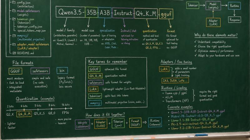
The problem is not that these names are badly chosen. It is that they describe things of completely different natures, stacked into a single filename. safetensors is a storage format. Q4_K_M is a compression method. A3B describes the model architecture. UD- is a vendor brand. mmproj is a separate component. 00001-of-00004 warns you that three more files are missing. All of it coexists with no visible hierarchy.
This article takes the stack apart, layer by layer. We start from what a downloadable model actually is, move up to file formats, then numeric precision, then quantization, and finish with the exotic labels nobody ever explains. By the end, you will be able to read the vast majority of names you will meet, and more importantly, know which one to download.
- 1. What You Are Actually Downloading
- 2. Anatomy of a Model Repository
- 3. Four Questions You Should Never Mix Up
- 4. File Formats
- 5. Numeric Precision, Before Even Talking About Quantization
- 6. Quantization: Compressing Without Breaking Everything
- 7. Decoding a GGUF Quantization Name
- 8. Ecosystem Labels:
UD-,UVMAX,Transcoded - 9. Decoding the Model Name Itself
- 10. Adapting a Model: LoRA vs Full Finetune
- 11. What to Choose, Concretely
- Key Takeaways
- Further Reading
1. What You Are Actually Downloading
1.1. A Model Is a Large Table of Numbers
When you download a language model, you are downloading neither a program nor a knowledge base in the classical sense. You are downloading weights: matrices of numbers, produced by training, that encode everything the model has learned.
Those blocks of numbers have a technical name that will keep coming back in this article: a tensor is an array of numbers, with one, two, or more dimensions. A model holds thousands of them, each labeled to show which layer and which function it serves, for instance model.layers.12.self_attn.q_proj.weight.
Those numbers mean nothing in isolation. They come alive only when a program (the runtime, or inference engine) loads them into memory and puts them to work in the right order. This is a fundamental distinction, and it explains half the confusion:
- The weights file is passive. It is data.
- The runtime (
llama.cpp, Ollama, vLLM, MLX, LM Studio…) is active. It is code.
A file format therefore does not determine speed on its own. Speed comes out of the meeting between the format, the numeric representation stored, the runtime, its kernels, and the hardware.
1.2. Parameters: The First Number to Look At
In Llama-3.1-8B or Qwen3.5-35B, the number followed by B means billions of parameters. It is how many numeric values the model stores.
That figure governs two things: the model’s capacity, and above all how much memory it takes to load it. The base formula is disarmingly simple:
Memory ≈ parameter count × bytes per parameter
A model with 8 billion parameters stored at 2 bytes each needs roughly 16 GB. At 4 bits, the theoretical figure is 4 GB; in practice a 4-bit quantization weighs more like 4.5 to 5 GB, because it also stores scale factors and keeps some tensors at higher precision. That is exactly what quantization does, and it is why quantization takes up half of this article.
One clarification that saves a lot of grief: this formula estimates the weight of the parameters, not the total memory needed to run the model. On top come the KV cache, the runtime buffers, temporary activations, and headroom for the system.
The three memory costs everyone forgets.
- The KV cache keeps the attention keys and values of the tokens already processed, so nothing has to be recomputed on each new token. It grows with context length and with the number of concurrent requests: this is what overflows on long contexts.
- The runtime buffers are the work areas the engine reserves at load time. Their size depends on the model, the backend, and the maximum context configured.
- Temporary activations are the intermediate results produced layer after layer. Their memory is recycled continuously, but their peak rises with the number of tokens processed together.
Budget around 20% on top of the weight of the weights for single-user use at moderate context. That is only an order of magnitude: at 100,000 tokens, the KV cache alone can run to several tens of gigabytes.
1.3. And a Commercial Model, How Much Does It Weigh?
The question comes naturally: if an 8B needs 16 GB, what would Claude Fable 5, GPT, or Gemini need? The honest answer is that only their makers know. Closed-model vendors publish neither the parameter count, nor the exact architecture, nor the precision used in production. Every figure in circulation is an estimate or an unverifiable leak, and quoting those as facts would be dishonest.
What we can do is calibrate the order of magnitude against the largest open-weight models, since the formula itself does not change:
| Model | Total parameters | Active per token | Published weights | If shipped in BF16 |
|---|---|---|---|---|
| Llama 4 Maverick | 400 billion | 17 billion | ~800 GB (BF16) | ~800 GB |
| DeepSeek-V4-Flash | 284 billion | ~13 billion | ~146 GB (mixed FP4/FP8) | ~570 GB |
| DeepSeek-V4-Pro | 1.6 trillion | ~49 billion | ~865 GB (mixed FP4/FP8) | ~3.2 TB |
| Kimi K3 | 2.8 trillion | 104 billion | ~1.56 TB (MXFP4) | ~5.6 TB |
Dense or MoE? Two ways to build a model, and two readings of the “active per token” column.
- A dense model puts all its parameters to work on every token. Total and active are the same number.
- A MoE model (Mixture of Experts) replaces some layers with a set of experts, specialized sub-networks. A small network called the router picks a few of them for each token; the rest stay idle.
Hence the two figures: total parameters dictate memory, since everything has to be loaded, and active parameters dictate compute. The naming of these models, of the 35B-A3B kind, is decoded further down.
Three lessons read straight off that table.
First, low precision is no longer a third-party operation: it is in the original release. DeepSeek-V4 ships in mixed FP4/FP8, Kimi K3 in MXFP4 obtained through quantization-aware training. Vendors no longer wait for someone else to compress their model, they ship the compressed version themselves.
Second, memory scales with the total, not with the active parameters. Kimi K3 activates only 104 billion parameters per token out of 2.8 trillion, under 4%, and you still have to load the full 1.56 TB. A MoE saves compute, not memory.
Third, the largest models are not always published. Meta’s Llama 4 Behemoth, announced at around 2 trillion parameters, never got public weights: it serves as a teacher model to distill Scout and Maverick.
A frontier proprietary model most likely sits in those waters, if not above them. At that scale the weights no longer fit on one machine: they are spread across several dozen interconnected datacenter GPUs, and the service is shared among thousands of concurrent users. That is what explains, beyond any licensing question, why you will not run Claude or GPT on your laptop: the memory gap with an 8B is a matter of hundreds of times.
The takeaway: the parameters × bytes per parameter formula admits no exception. A closed model does not escape physics, it only escapes publishing its numbers.
1.4. “Open Weights” Is Not “Open Source”
Marketing vocabulary maintains a confusion here that is worth clearing up immediately.
- An open weights model publishes its weights. You can download it, run it offline, adapt it. But the training data and the full training code are generally not published.
- An open source model in the sense of the OSI definition also provides the parameters, the code needed to train and run the system, and information about the data detailed enough that a skilled person could rebuild a substantially equivalent system. The definition does not require shipping the raw dataset, which is often locked up by copyright or privacy law. Some projects go further: AI2’s OLMo family also publishes its dataset, its logs, and hundreds of intermediate checkpoints under Apache 2.0.
Mistral AI sits at the other end of the spectrum, and it is the most instructive counter-example. Its models ship under Apache 2.0, in base and instruct versions, which is exactly as permissive as OLMo on the licensing axis. But the vendor states plainly that it does not disclose the datasets used for training, which it keeps as proprietary assets along with its training logic. Permissive licensing and data transparency are therefore two independent axes: Apache 2.0 tells you what you may do with the model, not how much you will know about it.
The difference is not merely theoretical, because it shows up in the license. Apache 2.0 and MIT are OSI-approved and allow commercial use, subject to light obligations: keeping copyright and license notices, plus a patent clause on the Apache 2.0 side. Custom licenses (the Llama Community License being the best-known example) may instead impose a user threshold beyond which permission becomes necessary, or restrict certain fields of use. The clauses shift from one version to the next: the Llama 3 license tightly constrained using outputs to improve another model, and the Llama 4 license relaxed that point. Read the exact version that applies to the model you are downloading.
Before building a product on a model, read its license, not its tagline. “Open” means nothing legally.
2. Anatomy of a Model Repository
Models are downloaded from the Hugging Face Hub, the ecosystem’s central catalog, whose filters by task, library, license, or format are the fastest way to track down a specific variant. Each model occupies a repository there, technically a Git repository backed by large-file storage, holding its files, its model card, and its version history.
Open any “standard” (non-quantized) repository and you will always find roughly the same thing:
config.json                        → the architecture blueprint
model-00001-of-00004.safetensors   → weights, chunk 1/4
model-00002-of-00004.safetensors   → weights, chunk 2/4
...
model.safetensors.index.json       → the map: which weight in which chunk
tokenizer.json                     → the text splitter
tokenizer_config.json              → its configuration, including the chat template
special_tokens_map.json            → the special tokens
generation_config.json             → default generation settings
README.md → the model card2.1. config.json: The Blueprint
This file describes the architecture: number of layers, vocabulary size, number of attention heads (for each word, they spot which other words in the text help make sense of it, such as what a pronoun refers to; each layer has several of them, working in parallel), internal dimensions. It is the assembly plan. Without it, the weights are just a pile of numbers nobody knows how to assemble.
It is also the file a runtime reads to determine whether it knows how to execute this model. When llama.cpp or vLLM tells you “unsupported architecture”, this is where it was decided.
2.2. Shards: Why Your Model Comes in Four Pieces
Large models are split into files of a few gigabytes, shards, named model-00001-of-00004.safetensors. This is not a variant, it is one logical file, cut up. You need all of them.
The model.safetensors.index.json file holds the map (weight_map) telling which tensor lives in which chunk. The same logic exists on the GGUF side, where files are named ...-00001-of-00003.gguf.
As of this writing, Ollama does not always load a split GGUF directly, depending on how it was distributed and which version you run. Merging the pieces first with llama-gguf-split --merge may be necessary. LM Studio, on the other hand, handles them natively.
2.3. The Tokenizer: The Interpreter
A model does not read text. It reads integers. The tokenizer does the translation both ways: it splits your sentence into tokens (word fragments), converts them into numeric identifiers, and does the reverse trip on the way out.
It is a component separate from the weights, but just as indispensable. Served with an incompatible tokenizer, a model may produce gibberish, or suffer a major quality drop without becoming unreadable.
2.4. The Chat Template: The Most Common Trap
Hidden inside tokenizer_config.json, or in a dedicated file depending on the repository, is often a chat template: the exact mold that turns a conversation into a single string, with the right role markers and the right control tokens.
This is a frequent trap. With the right tokenizer but the wrong chat template, an excellent model stays perfectly readable while following instructions very poorly, simply because the prompt was sent in the wrong mold or because a <bos> token was duplicated. Hence the rule:
from transformers import AutoTokenizer

tok = AutoTokenizer.from_pretrained("Qwen/Qwen3-0.6B")
messages = [{"role": "user", "content": "Hello"}]

# Always use this...
inputs = tok.apply_chat_template(messages, tokenize=True, add_generation_prompt=True)

# ...rather than assembling the prompt string by hand.3. Four Questions You Should Never Mix Up
This is the heart of the article. Most misunderstandings come from the fact that a single filename answers four independent questions at once. Separate them, and everything becomes readable.
| Question | What it describes | Example answers |
|---|---|---|
| What is it stored in? | The file format, the container | safetensors, GGUF, ONNX, .pt |
| At what precision? | Bits per weight | BF16, FP8, Q4_K_M, NF4, MXFP4 |
| How is it specialized? | The adaptation method | base model, Instruct, LoRA, full finetune |
| What runs it? | The target runtime | llama.cpp, vLLM, MLX, ONNX Runtime |
A workable analogy: the format is the suitcase; quantization is how you fold and compress the clothes; the adapter is an accessory kit you add without rebuilding the wardrobe; a full finetune rebuilds the entire wardrobe; and the tokenizer is the language you speak once you arrive.
A model’s typical life cycle follows that same order:
Training                  Adaptation              Compression            Conversion
     │                          │                        │                     │
     ▼                          ▼                        ▼                     ▼
BF16 checkpoint   ──►   LoRA / full finetune   ──►  quantization    ──►   GGUF / MLX
(safetensors)             (adapter or               (Q4_K_M, AWQ,          (deployment
full checkpoint) NF4, MXFP4…) container)Each step is optional and independent of the others. That is why one model exists in dozens of variants.
Classic mistake #1: believing “GGUF” is a quantization. It is not: GGUF is a container, and it can hold unquantized weights (F16) just as well as Q4_K_M.
Classic mistake #2: believing “MLX” is a file format comparable to GGUF. It is not: MLX is a framework and a toolchain; MLX repositories are, in practice, safetensors.
4. File Formats
4.1. Safetensors: The De Facto Standard
This is the default format of the Hugging Face ecosystem, and the one a large share of models ship in at release.
Its structure is deliberately minimal: 8 bytes stating the header size, then a JSON header describing each tensor (name, shape, type, offset), then the raw tensor bytes, back to back, with no gaps.
┌────────────┬─────────────────────────┬──────────────────────────┐
│  8 bytes   │   JSON header           │   raw data               │
│  header    │   {"model.layers.0...": │   (contiguous tensors)   │
│  size      │    {dtype, shape,       │                          │
│            │     data_offsets}}      │                          │
└────────────┴─────────────────────────┴──────────────────────────┘Its name comes from its main selling point: safety. PyTorch’s historical format (.pt, .bin, .pth) relies on pickle, Python’s serialization mechanism, which can trigger arbitrary code execution on load. The risk narrowed considerably with PyTorch 2.6, where torch.load() defaults to weights_only=True and sharply restricts what the deserializer accepts. It comes back as soon as you switch to weights_only=False. Safetensors, by contrast, contains only data: there is nothing to execute.
On top of that come concrete guardrails: the header is capped at 100 MB to prevent denial-of-service attacks, and byte ranges are guaranteed not to overlap. Finally, loading is very fast because tensors can be read via mmap, with no intermediate copy.
Prefer the safetensors variant when it exists. Only load an old PyTorch checkpoint from a source you trust, and be wary of code that forces weights_only=False to “make loading work”.
4.2. GGUF: The Local Format
GGUF (GGML Universal File) is the format of the llama.cpp family, and by extension that of Ollama, LM Studio, Jan, KoboldCpp, and most local inference tools.
Four design properties explain its success:
- Self-contained in the common case: weights, metadata and tokenizer fit in the same file. One
.ggufis then enough to run the model, with noconfig.jsonalongside and no repository to clone. Very large models are still split across several GGUFs, however, and multimodal models come with a companion file. - Typed key-value metadata: the format is extensible without breaking backward compatibility.
mmaploading: the model is memory-mapped rather than read in one pass, which avoids copies and shortens startup. The first reads still cause page faults, and the runtime still has to initialize its structures.- Optimized for inference, not for training.
In exchange, GGUF is tightly bound to its ecosystem. A model exists in GGUF only if its architecture has been implemented in llama.cpp. That is why GGUFs for a freshly released model sometimes arrive a few days after the safetensors.
# The official chain: safetensors → GGUF → quantized GGUF → execution
python convert_hf_to_gguf.py --outfile model-bf16.gguf --outtype bf16 --remote <hf_repo>
./build/bin/llama-quantize model-bf16.gguf model-Q4_K_M.gguf Q4_K_M
./build/bin/llama-cli -m model-Q4_K_M.gguf -p "Hello"Note the second line carefully: quantization is a separate step, applied to a GGUF. That is the proof that GGUF is not a quantization. That said, running a GGUF assumes two things: that the runtime knows its architecture, and that it can read its quantization type.
4.3. MLX Repositories: The Apple Silicon Path
MLX is Apple’s compute framework for its own chips, designed around unified memory and accelerated by Metal. mlx-lm is its Python package dedicated to language models: generation, conversion, quantization, fine-tuning, and an HTTP server.
An important point to avoid the misreading: MLX is not a file format. It is a framework plus a toolchain. The MLX repositories you find on the Hub (the mlx-community organization hosts several thousand) are in practice safetensors, along with a configuration describing the MLX quantization scheme (often 4-bit with a group size of 64).
# Convert a Hugging Face model into a quantized MLX repository
python -m mlx_lm.convert --hf-path mistralai/Mistral-7B-v0.1 -q

# Generate text
python -m mlx_lm.generate --model mlx-community/Mistral-7B-Instruct-v0.3-4bit --prompt "Hello"

# Serve an OpenAI-compatible API
mlx_lm.server --model mlx-community/Mistral-7B-Instruct-v0.3-4bitThe compatibility lock here is mostly hardware, but it has shifted. mlx-lm is still designed and documented first and foremost for Apple Silicon, and that is where the mlx-community ecosystem makes sense. The MLX framework itself has since gained a CUDA backend and a CPU variant for Linux; it is Metal acceleration that requires a Mac.
4.4. ONNX: Industrial Portability
ONNX is of another nature: it stores not just weights, but a compute graph plus weights. That makes it portable across very different runtimes and hardware (CPU, GPU, NPU, embedded accelerators) and enables aggressive optimization through ONNX Runtime.
It is the format you meet in embedded production, edge computing, and industrial inference chains. For local LLMs on a workstation, it is markedly less convenient than GGUF: more engineering, fewer ready-to-run models.
4.5. Format Recap
| Format | Nature | Bundles the tokenizer? | Typical ecosystem | Good for |
|---|---|---|---|---|
| Safetensors | Tensor container | No (separate files) | Hugging Face, PyTorch, vLLM, MLX | Starting point, training, GPU servers |
| GGUF | Self-contained container | Yes | llama.cpp, Ollama, LM Studio | Local inference, CPU and consumer GPU |
| ONNX | Graph + weights | No | ONNX Runtime, embedded | Cross-hardware portability, edge production |
.pt / .bin | pickle serialization | No | Legacy PyTorch | Old checkpoints and resuming training in a controlled environment; not advised for distributing weights |
5. Numeric Precision, Before Even Talking About Quantization
Before tackling Q4_K_M and friends, you need the layer underneath: how many bits do we use to store a number?
5.1. Floating-Point Formats
| Format | Size | What to remember |
|---|---|---|
| FP32 | 4 bytes | The historical reference precision. Now rare for LLMs: too expensive. |
| FP16 | 2 bytes | Half the memory, but a narrow value range: overflow risk during training. |
| BF16 | 2 bytes | Same exponent range as FP32, less mantissa. More robust than FP16 for training. This is the native format of most published models. |
| FP8 | 1 byte | Twice as compact as BF16, natively supported by recent GPUs. |
| FP4 | 0.5 byte | The low frontier of floating point. Requires per-block scaling mechanisms (see below). |
The FP16 / BF16 difference deserves a second of attention because it comes up often. Both take 2 bytes. FP16 splits those 16 bits into 5 exponent bits and 10 mantissa bits; BF16 into 8 exponent bits and 7 mantissa bits. BF16 therefore sacrifices fineness to preserve the same value amplitude as FP32, which avoids exploding and vanishing gradients during training. That is why it won.
5.2. The Memory Rule
This is the single most useful calculation in the whole article:
| Precision | Bytes / parameter | 8-billion model | 70-billion model |
|---|---|---|---|
| FP32 | 4 | ~32 GB | ~280 GB |
| BF16 / FP16 | 2 | ~16 GB | ~140 GB |
| FP8 / INT8 | 1 | ~8 GB | ~70 GB |
| 4-bit | ~0.5 to 0.6 | ~4.5 to 5 GB | ~40 GB |
4-bit is never exactly 0.5 byte per parameter. You have to add the scale factors stored for each block of weights. llama.cpp’s Q4_K_M actually weighs about 4.89 bits per weight, or ~0.61 byte. That is precisely why an 8B model in Q4_K_M is ~4.9 GB and not 4 GB.
And that is only the model weights. On top comes the KV cache, which grows with context length and can account for several gigabytes on a long context. Always budget headroom.
6. Quantization: Compressing Without Breaking Everything
6.1. The Principle
Quantizing means storing weights on fewer bits. A weight that took 16 bits now takes 4. Memory is divided by four.
But you cannot simply truncate: everything would be lost. The universal trick is block-wise (or group-wise) quantization. Weights are cut into small groups (typically 32, 64, or 128 values) and for each group you store:
- the values, coded on few bits (the index into a reduced scale);
- one or two scale factors, stored at higher precision, which let you reconstruct the order of magnitude.
Original weights (BF16):  [ 0.031  -0.128   0.094  ...  -0.011 ]   ← 16 bits each
                                        │
                          block of 32 values + 1 scale
                                        ▼
Quantized weights (4-bit): [ 5 1 12 ... 7 ] + scale=0.0104 ← 4 bits eachThis is where the word block comes from, and it is also where a frequent ambiguity comes from. If a model card mentions “group size 64” or “block size 128”, it is about quantization. If it says “32 blocks” or “32 layers”, it is about Transformer architecture, where a block means a full layer (attention + feed-forward network). Two meanings, no relation.
6.2. When Do We Quantize? PTQ vs QAT
Two strategies coexist:
- PTQ (Post-Training Quantization): quantize after training. Fast, requires only a little calibration data, sometimes none. This is what produces the vast majority of quantized models you download.
- QAT (Quantization-Aware Training): simulate quantization during training (fake quantization), so the model learns to be robust to precision loss. Considerably more expensive, but considerably more faithful at very low precision.
For a user, the distinction is readable on the model card. A model published as QAT by its original vendor will generally beat, at equal size, a third-party PTQ quantization.
6.3. The Main Quantization Families
One vocabulary trap to clear up first: these names do not all denote the same category of thing. Some are coding schemes, others algorithms, others still a library or a storage format. Hence the second column.
| Name | Nature | In plain terms | Where you meet it |
|---|---|---|---|
| k-quants Q4_K_M… | GGUF coding scheme | Not every tensor gets the same number of bits: those that tolerate imprecision badly keep more. | llama.cpp, Ollama, LM Studio |
| IQ-quants IQ4_XS… | GGUF coding scheme | Same principle, but a calibration pass first measures which weights actually matter. Smaller than a k-quant at comparable quality, especially below 4 bits. | llama.cpp, Ollama, LM Studio |
| GPTQ | Compression algorithm | Works through the model layer by layer, correcting the errors already introduced as it goes. | PyTorch, vLLM |
| AWQ | Compression algorithm | Spots the weights that receive the strongest signals and leaves them more precision. | vLLM, TensorRT-LLM |
| bitsandbytes NF4, LLM.int8()… | Python library | Compresses the model at load time, with no compressed file to prepare in advance. The short path to QLoRA. | Transformers, PEFT |
| compressed-tensors | Storage format | Compresses nothing on its own: it lets a safetensors repository hold weights compressed by various methods. | vLLM, LLM Compressor |
A word on the 2026 landscape: AWQ has become very common for new releases on the GPU server side, carried by better quality and faster kernels than GPTQ, while GGUF is one of the dominant formats for local inference. GPTQ remains used and supported by several runtimes; what moves is mostly its implementations, with AutoGPTQ gradually giving way to GPTQModel. A recent model typically ships as BF16 safetensors first, then as GGUF and AWQ in the following days.
6.4. The FP4 Formats: MXFP4 and NVFP4
Newcomers, and increasingly visible now that hardware supports them natively. Kimi K3 is the most spectacular illustration: its 2.8 trillion parameters ship directly in MXFP4, with MXFP8 activations and quantization learned from the SFT stage onward. Both formats encode weights in E2M1 (4 bits: 1 sign, 2 exponent, 1 mantissa), but differ on the scaling mechanics:
| MXFP4 | NVFP4 | |
|---|---|---|
| Block size | 32 values | 16 values |
| Scale | one per block, in E8M0 | one per block in FP8 (E4M3) + one per tensor in FP32 |
| Governance | Open OCP standard, backed by AMD, Arm, Intel, Meta, Microsoft, NVIDIA, Qualcomm | NVIDIA format, tailored to Blackwell’s FP4 cores |
| Takeaway | Multi-vendor, portable | Finer blocks and dual scaling: better fidelity, but tied to NVIDIA |
In practice: the 16-value blocks and dual scaling give NVFP4 a finer granularity, while MXFP4 bets on multi-vendor portability. Their relative quality depends on the model, the calibration pipeline, the kernels, and the task. Do not treat them as automatic substitutes for FP8 or BF16: compare them on your real workloads, especially reasoning and long contexts.
7. Decoding a GGUF Quantization Name
Time to read the labels. Let us take Q4_K_M apart, piece by piece.
Q  4  _  K  _  M
│  │     │     │
│  │     │     └── variant: S (small), M (medium), L (large)
│  │     └──────── "k-quant" family
│  └────────────── bits per weight
└───────────────── QuantizedQ: the tensor is quantized (as opposed toF16orBF16).- The digit: the order of magnitude of compression.
Q2throughQ8. The lower it is, the smaller the file and the more quality degrades. K: the k-quant family, which does not apply the same precision everywhere. Tensors deemed sensitive get more bits.S/M/L: the variant within the family (small, medium, large). These are not three notches on a uniform slider, but three recipes that distribute quantization types across tensors differently.
The IQ prefix (IQ4_XS, IQ3_XXS, IQ2_M…) marks the second family: importance-aware quantizations. They rely on an importance matrix (imatrix), computed by running a calibration dataset through the model to measure which weights actually matter. The result: at comparable quality, they are smaller than k-quants, especially at very low bit rates. Their decoding speed, on the other hand, depends heavily on the processor, the instruction sets available, and the backend. Measure it on your machine rather than assuming it.
The full list offered by llama-quantize, from most aggressive to most faithful:
2-bit    IQ1_S  IQ1_M  IQ2_XXS  IQ2_XS  IQ2_S  IQ2_M  Q2_K_S  Q2_K
3-bit    IQ3_XXS  IQ3_XS  IQ3_S  IQ3_M  Q3_K_S  Q3_K_M  Q3_K_L
4-bit    IQ4_XS  IQ4_NL  Q4_K_S  Q4_K_M
5-bit    Q5_K_S  Q5_K_M
6-bit+ Q6_K Q8_0 F16And the most widely shared practical recommendation:
Q4_K_M remains an excellent starting point, particularly while you have no measurement specific to your model and your hardware. Move up to Q5_K_M or Q6_K if quality matters most and memory allows. Drop to Q3_K_M or Q2_K only if you have no choice. Below 3 bits, degradation generally becomes noticeable on reasoning tasks.
A useful heuristic: a bigger model heavily quantized often beats a small model lightly quantized, at equal memory. A 30B in Q4_K_M frequently wins against an 8B in Q8_0. It is not a guarantee: the trend sometimes reverses on code, under-represented languages, or long contexts. Compare on your real tasks.
8. Ecosystem Labels: UD-, UVMAX, Transcoded
Beyond the standard formats, you will run into names that appear in no specification. These are neither formats nor standards: they are vendor-specific quantization recipes. Treating them as pipeline labels, not as interoperability promises, is the right stance.
8.1. UD-Q4_K_XL: Unsloth Dynamic
The UD- prefix stands for Unsloth Dynamic. The principle: instead of applying a uniform scheme, the method analyzes each layer and picks for it the quantization type that minimizes loss, helped by a calibration pass. A UD-Q4_K_XL therefore mixes several types and preserves some tensors at higher precision; the exact split depends on the recipe built for that particular model.
Two consequences:
- The gain is sharpest at very low precision (
Q2,Q3), where uniform quantization breaks the model. - The
XLsuffix is not part of the GGUF specification. It is a naming convention specific to Unsloth, denoting a variant with a more generous precision budget.
These files remain standard GGUFs: they load in llama.cpp and the tools built on it, with no special handling.
8.2. UVMAX: kernelpool
Another in-house scheme. In certain kernelpool MLX repositories, such as kernelpool/Kimi-K3-2bit-UVMAX, UVMAX denotes a mixed-precision recipe: bit widths are assigned per tensor class, based on the quantization error measured for each, rather than uniformly. Feed-forward experts are compressed aggressively there, while sensitive components (routers, attention, lm_head) are preserved at higher precision. This is not a standard, and nothing guarantees the label covers the same recipe elsewhere.
This is case-by-case quantization. The quality gain at a given size can be real. In exchange, portability is low: these repositories target a specific runtime, often mlx-lm or mlx-vlm, and sometimes require an unreleased development version.
8.3. Transcoded
The term has no standard definition. In some current MLX repositories, it describes converting NVFP4 checkpoints, produced for NVIDIA hardware, into a representation MLX can use, while trying to preserve the original quantization logic. Elsewhere it may simply mean “reconverted from another format”.
It is therefore not a compression method but a conversion operation. The question to ask is not “is it good?” but “for which runtime?”.
General rule for any exotic label: ask yourself four questions before downloading. What is the actual container? What is the target runtime? What minimum versions? Which tokenizer? If the model card does not answer, move on.
9. Decoding the Model Name Itself
The model name, before any quantization suffix, already encodes a lot of information.
Qwen3.5  -  35B  -  A3B  -  Instruct  -  GGUF
    │        │       │         │           │
    │        │       │         │           └─── distribution format
    │        │       │         └─────────────── training type
    │        │       └───────────────────────── active parameters (MoE)
    │        └───────────────────────────────── total parameters
└────────────────────────────────────────── family and versionThis name is a teaching composite: it strings together segments you will not always see side by side. The official repository is called Qwen/Qwen3.5-35B-A3B, with a -Base variant; the Instruct suffix, meanwhile, is a very widespread convention elsewhere.
9.1. Base, Instruct, Chat
- Base (or no suffix): the raw model, trained only to predict the next token. It can technically answer or continue a conversation, but its behavior is less predictable and far less suited to assistant use. It is the starting point for fine-tuning.
- Instruct / Chat / IT: the model has been instruction-tuned. This is the one you want for conversation or for following directions.
Picking a Base model while thinking you are getting an assistant is one of the most common early disappointments.
9.2. Thinking, Reasoning
The model goes through a reasoning phase before its final answer. Depending on the model and how it is run, that phase is either generated explicitly between dedicated tags, or stays partly hidden and summarized by the runtime. Better on logic, math, and code tasks, at the cost of far more generated tokens, hence latency and context memory.
9.3. A3B and Mixture-of-Experts Models
Two numbers in a name (35B-A3B) signal a MoE (Mixture of Experts) architecture: the model holds 35 billion parameters in total but activates only 3 billion per token.
The practical consequence is counter-intuitive and worth remembering:
- Memory scales with the total (35B): everything must be loaded.
- Compute per token is far below that of a dense 35B model, since only a fraction of the experts fires.
Do not conclude from this that a 35B-A3B will run as fast as a dense 3B. Shared layers, attention, the router, how many experts activate, the volume of memory reads, and the quality of the backend’s MoE kernels all bear on real throughput. A MoE buys you saved compute, not saved memory.
9.4. Distill
The model was trained to imitate a larger model: this is knowledge distillation. A DeepSeek-R1-Distill-Qwen-7B is not a shrunken R1: it is a Qwen 7B trained on R1’s outputs. It inherits part of the behavior, not the architecture.
9.5. Abliterated, Uncensored
These two labels are not synonyms, and conflating them leads to surprises.
Abliterated denotes a family of weight-editing techniques aimed at reducing the internal directions associated with refusal. You measure the difference in activations between harmless prompts and refused prompts, then subtract that direction from the weights. This is not a prompt-level workaround: it is a permanent modification, with possible side effects on the model’s other capabilities.
Uncensored is far vaguer. Depending on the repository, the label may cover an ablation, a fine-tune on a different dataset, a mere system-prompt change, or a purely commercial promise. Read the model card before concluding anything.
9.6. mmproj: Multimodal Models
A multimodal model accepts more than text as input, most often images, sometimes audio or video, and answers in text. That is what lets you hand it a photo or a screenshot and ask questions about it.
In most multimodal GGUF distributions, the language model comes with a separate file, still called mmproj by tradition (mmproj-F16.gguf). It carries the projection that brings the image into a space the language model understands, and depending on the architecture other pieces of the vision encoder along with preprocessing parameters.
llama-server -m gemma-3-4b-it-Q4_K_M.gguf --mmproj mmproj-gemma-3-4b-it-F16.ggufForgetting --mmproj leaves you with a model that sees nothing.
10. Adapting a Model: LoRA vs Full Finetune
The last layer of vocabulary: how do you specialize a model?
10.1. The Full Finetune
You continue training the model on specific data, updating all the weights. Maximum control, deep adaptation, but every variant produces a complete checkpoint, as heavy as the original model. Expensive to train, expensive to store, expensive to distribute.
10.2. LoRA and Adapters
The parameter-efficient approach flips the logic: you freeze the base model and train only small modules grafted onto it. LoRA (Low-Rank Adaptation) is the dominant variant.
The result fits in two files:
adapter_config.json           → which base model, which rank, which layers targeted
adapter_model.safetensors → the adapter weightsAnywhere from a few megabytes to several hundred depending on the rank, the modules targeted, and the precision, against several gigabytes for a full checkpoint. You can store dozens of them, load them on demand, swap them.
from peft import LoraConfig, get_peft_model

config = LoraConfig(
    r=16,
    lora_alpha=32,
    target_modules=["q_proj", "k_proj", "v_proj", "o_proj"],
    lora_dropout=0.05,
    task_type="CAUSAL_LM",
)
model = get_peft_model(base_model, config)
# ... training ...
model.save_pretrained("./my_adapter")The constraint: an adapter is unusable without its exact base model. If you download an adapter_model.safetensors without reading which model it targets, you have downloaded a key ring with no lock.
10.3. QLoRA
The combination that democratized fine-tuning: load the base model quantized to 4-bit (typically NF4, with double quantization), frozen, and train a LoRA adapter on top at higher precision.
The model takes a quarter of its usual memory, and only the adapter’s few million parameters receive gradients. This is what makes it possible to adapt a model of several tens of billions of parameters on a single GPU.
from transformers import AutoModelForCausalLM, BitsAndBytesConfig

cfg = BitsAndBytesConfig(
    load_in_4bit=True,
    bnb_4bit_quant_type="nf4",
    bnb_4bit_use_double_quant=True,
)
model = AutoModelForCausalLM.from_pretrained(
    "meta-llama/Llama-3.1-8B",
    device_map="auto",
    quantization_config=cfg,
)10.4. Merge or Not
An adapter can stay separate, with the runtime loading it on top of the base, or be merged into the model weights to produce a standalone checkpoint.
Contrary to a widespread belief, staying separate works on the GGUF side too. llama.cpp can convert a PEFT adapter into a GGUF adapter, then apply it to a base model with --lora or --lora-scaled. You can even load several at once and tune their weight, without rewriting anything.
python convert_lora_to_gguf.py ./my_adapter --base ./base_model
llama-cli -m model-Q4_K_M.gguf --lora my_adapter-F16.gguf -p "Hello"Merging keeps its uses: shipping a single artifact, or targeting a runtime that does not handle separate adapters.
11. What to Choose, Concretely
11.1. The Decision Tree
I just want to RUN a model
│
├── On an Apple Silicon Mac
│   └── MLX 4-bit repository  (mlx-community/…-4bit)
│       └── model < 7B or quality critical? → MLX 8-bit
│
├── On PC / Linux, CPU or consumer GPU
│   └── GGUF Q4_K_M  ← the robust default
│       ├── more RAM available?        → Q5_K_M or Q6_K
│       ├── memory very tight?         → IQ3_M or Q3_K_M
│       └── maximum local quality?     → Q8_0
│
└── On a GPU server, multiple users
    └── AWQ or compressed-tensors via vLLM

I want to ADAPT a model
│
├── Limited GPU budget       → QLoRA (4-bit base + LoRA adapter)
├── Comfortable budget       → LoRA on a BF16 base
└── Deep transformation → full finetune11.2. Summary Table
| Option | Size (8B model) | Quality | Hardware | Ease |
|---|---|---|---|---|
| Safetensors BF16 | ~16 GB | Reference | GPU, large servers | Simple on HF, heavy on RAM |
GGUF Q8_0 | ~8.5 GB | Near-identical to BF16 | CPU/GPU with comfortable RAM | Very simple |
GGUF Q5_K_M / Q6_K | ~5.7 to 6.6 GB | Very good | CPU/consumer GPU | Very simple |
GGUF Q4_K_M | ~4.9 GB | Good, minimal loss | CPU/consumer GPU | Very simple: the default |
GGUF IQ3_M / Q3_K_M | ~3.7 to 4 GB | Visible degradation | Constrained machines | Simple, verify results |
GGUF Q2_K | ~3 GB | Clear degradation | Last resort | Avoid unless necessary |
| MLX 4-bit | ~4.5 GB | Good | Mainly Apple Silicon via mlx-lm | Very simple on Mac |
| AWQ 4-bit | ~5.5 GB | Good, fast kernels | NVIDIA GPU | Good vLLM integration |
| LoRA (adapter alone) | a few MB to several hundred | Depends on training | Same as the base | Simple, but base required |
Sizes are orders of magnitude for a dense 8-billion-parameter model; they vary with architecture, notably vocabulary size.
Key Takeaways
The ecosystem’s confusion comes down to one fact: very similar words denote things of different natures. Once the separation is made, everything falls into place.
- GGUF, Safetensors, ONNX answer “what is it stored in”. They are containers.
Q4_K_M,NF4,AWQ,MXFP4,UVMAXanswer “how many bits”. They are quantization schemes.- Base, Instruct, LoRA, finetune answer “how is it specialized”.
llama.cpp, vLLM, MLX, ONNX Runtime answer “what runs it”.- The tokenizer and chat template fit in none of those boxes, and break everything when neglected.
To get started without missteps, four decisions are enough:
- Pick the hardware first. Apple Silicon Mac → MLX. Everything else → GGUF via
llama.cpp, Ollama, or LM Studio. - Take
Q4_K_M(or MLX 4-bit) as your starting point, and deviate only with a measured reason. - Check the tokenizer and chat template before concluding a model is bad. Very often, the prompt is malformed.
- Treat
UD-,UVMAX,Transcodedand friends as vendor labels. They can be excellent, but they require reading the model card, not the filename.
The rest (IQ3_XXS, NVFP4, A3B, mmproj) stops being jargon once you know which question each term answers.
In one sentence: the format is the suitcase, quantization is how you fold, the adapter is the accessory kit, and the tokenizer is the language you speak once you arrive.
Further Reading
- GGUF specification: ggml
llama-quantizequantization types- Safetensors: format and specification
- MLX LM: documentation
- Unsloth Dynamic 2.0 GGUFs
- PEFT: Parameter-Efficient Fine-Tuning
- Multimodal support in
llama.cpp - Open Compute Project: Microscaling Formats (MX)
- The Open Source AI Definition 1.0: OSI
torch.load: security andweights_only- LoRA adapters in GGUF with
llama.cpp - MLX: installation and available backends
- Official Qwen3.5-35B-A3B model card
- Official Kimi K3 model card
- Quantization in Transformers: AWQ, GPTQ, compressed-tensors